Residual Neural Networks

Introduction

This type of neural network, often abbreviated as ResNet, was introduced by He et al. (2015). We will discuss the motivation for and architecture of these networks, and their relation to ODEs. This will naturally lead to the concept of neural ODEs.

Vanishing Gradients

Consider a neural network with several layers $\ell = 1,\ldots,L$. Each layer $\ell$ has its own weights $\mathbf{W}_\ell = (W_\ell, b_\ell)$. During training, we optimize the loss function $\mathcal{L}$. If the network is very deep, say $L > 20$, and for the gradient of $\mathcal{L}$ it holds that

then the contribution of the first $\bar{\ell}$ layers is negligible as the influence of their weights on $\mathcal{L}$ is small. This leads to a cut-off in depth and the benefit in terms of generalization capabilities of deep networks is lost.

He et al. (2015) demonstrate that taking a deeper network can actually lead to an increase in training and testing error.

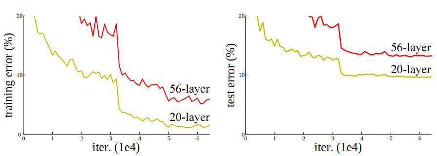
Thus, beyond a certain point, increasing the depth of a network can be counterproductive. Given this, we would like to come up with a network architecture that addresses the problem of vanishing gradients by ensuring that

This means requiring that when the weights of the network approach small values, the network should approach the identity mapping, and not the null mapping.

ResNet Architecture

The problem of vanishing gradients outlined above is alleviated by introducing a deep residual learning framework. Instead of hoping that each few stacked layers directly fit a desired underlying mapping, we explicitly let these layers fit a residual mapping. Formally, denoting the desired underlying mapping as $\mathcal{H}(x)$, we let the stacked nonlinear layers fit another mapping of $\mathcal{F}(x) \coloneqq \mathcal{H}(x) − x$. The original mapping is recast into $\mathcal{F}(x)+x$. It is easier to optimize the residual mapping than to optimize the original, unreferenced mapping. To the extreme, if an identity mapping were optimal, it would be easier to push the residual to zero than to fit an identity mapping by a stack of nonlinear layers.

The formulation of $\mathcal{F}(x) + x$ can be realized by feedforward neural networks with "shortcut connections" skipping one or more layers forming so-called residual blocks. In our case, the shortcut connections simply perform identity mapping, and their outputs are added to the outputs of the stacked layers.

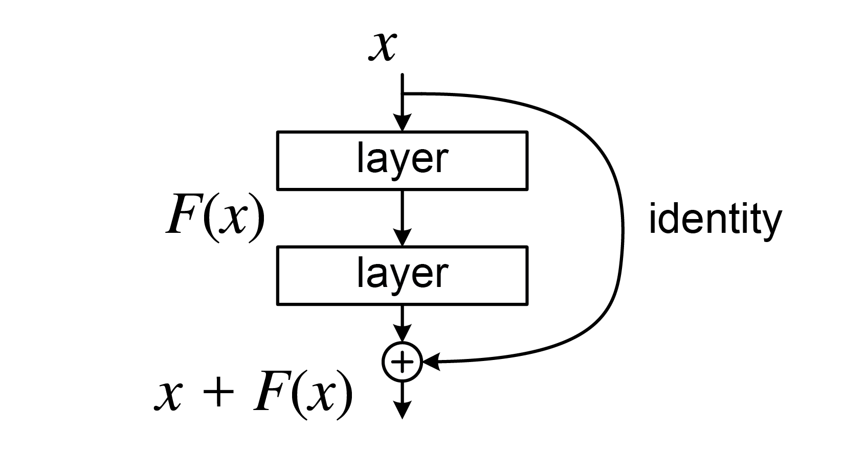
Identity shortcut connections neither add extra parameter nor computational complexity. The entire network can still be trained end-to-end with backpropagation, and can be easily implemented using common libraries without modifying the solvers.

Comparing Performance

To illustrate this we implement a simple fully connected neural network in Flux.jl.

using Flux
using BenchmarkTools: @benchmark

actual(x) = x

x_train = hcat(-10:10...)
y_train = actual.(x_train)

dense = Chain(
    Dense(1 => 1, tanh),
    Dense(1 => 1, tanh),
    Dense(1 => 1, tanh),
    Dense(1 => 1, identity),
)

loader = Flux.DataLoader((x_train, y_train), batchsize=8, shuffle=true);

function loop(model)
    optim = Flux.setup(Adam(), model)

    for epoch in 1:10_000
        Flux.train!(model, loader, optim) do m, x, y
            y_hat = m(x)
            Flux.mse(y_hat, y)
        end

        Flux.mse(model(x_train), x_train) < 0.01 && break
    end

end

@benchmark loop(dense)

BenchmarkTools.Trial: 3010 samples with 1 evaluation.
 Range (min … max):  124.333 μs … 15.881 ms  ┊ GC (min … max):  0.00% … 52.93%
 Time  (median):       1.139 ms              ┊ GC (median):     0.00%
 Time  (mean ± σ):     1.659 ms ±  1.938 ms  ┊ GC (mean ± σ):  18.10% ± 15.30%

    ▁▆█▆▄▂                                                      
  ▃▇███████▆▅▅▄▃▃▃▃▃▃▂▂▂▂▂▂▂▂▂▂▂▂▂▁▂▁▂▂▂▁▁▁▂▁▂▁▁▁▂▂▂▂▂▂▂▂▂▂▂▂▂ ▃
  124 μs          Histogram: frequency by time         10.8 ms <

 Memory estimate: 169.88 KiB, allocs estimate: 2050.

Comparing these benchmark results to a residual network with the same amount of layers reveals the benefits of these skip connections.

resnet = Chain(
    SkipConnection(
        Chain(
            Dense(1 => 1, tanh),
            Dense(1 => 1, tanh),
            Dense(1 => 1, tanh),
        ),
        +
    ),
    Dense(1 => 1, identity),
)

@benchmark loop(resnet)

BenchmarkTools.Trial: 10000 samples with 1 evaluation.
 Range (min … max):   88.465 μs …  10.694 ms  ┊ GC (min … max):  0.00% … 82.72%
 Time  (median):      93.265 μs               ┊ GC (median):     0.00%
 Time  (mean ± σ):   113.836 μs ± 406.215 μs  ┊ GC (mean ± σ):  15.60% ±  4.33%

   ▁▃▆▇███▇▆▅▄▃▂▁                        ▁▁▁ ▁                  ▂
  ▄█████████████████████▇█▇▆▆▇▇██▆▇▇████████████▇▇▆▆▇▇▆▇▆▆▆▆▅▅▅ █
  88.5 μs       Histogram: log(frequency) by time        130 μs <

 Memory estimate: 104.50 KiB, allocs estimate: 1197.

Connections With ODEs

Let us first consider a residual block with a single linear layer which can be mathematically formulated in the following manner

This can easily be rewritten as

for some scalar $\Delta t$.

Now consider a first-order system of (possibly nonlinear) ODEs, where given the IVP

we want to find $x(T)$. In order to solve this numerically, we can uniformly divide the temporal domain with a time-step $\Delta t$ and temporal nodes $t_\ell = \ell \Delta t, 0 \leq \ell \leq L+1$, where $(L+1)\Delta t = T$. Define the discrete solution as $x_\ell = x(\ell \Delta t)$. Then, given $x_{\ell-1}$, we can use a time-integrator to approximate the solution $x_\ell$. We can consider a method motivated by the forward Euler integrator, where the LHS of (1) is approximated by

The RHS is approximated using a parameter $\theta_\ell$ as

where we allow the parameters to be different at each time-step. Putting these two together, we get exactly the relation of the ResNet. In other words, a ResNet is nothing but a discretization of a nonlinear system of ODEs. We make some comments to further strengthen this connection.

• In a fully trained ResNet we are given $x(0)$ and the weights of a network, and we predict $x(L+1)$. In a system of ODEs, we are given $x(0)$ and $V(x,t)$, and we predict $x(T)$.

• Training the ResNet means determining the parameters $\theta$ of the network so that $x_{L+1}$ is as close as possible to $y_j$ when $x_0 = x_j$ for $j=1,\ldots,N_{\text{train}}$. When viewed from the analogous ODE point of view, training means determining the RHS $V(x,t)$ by requiring $x(T)$ to be as close as possible to $y_j$, when $x(0) = x_j$ for $j=1,\ldots,N_{\text{train}}$.

• In a ResNet we are looking for a single $V(x,t)$ that will map $x_j$ to $y_j$ for all $1\leq j \leq N_{\text{train}}$.

Neural ODEs

Motivated by the connection between ResNets and ODEs, neural ODEs were proposed by Chen et al. (2019). Consider a system of ODEs given by

Given $x(0)$, we wish to find $x(T)$. The RHS, i.e., $V(x,t)$, is defined using a feed-forward neural network with parameters $\theta$. The input to the network is $(x,t)$ while the output is $V(x,t)$ having the same dimensions as $x$. With this description, the system (2) is solved using a suitable time-marching scheme, such as forward Euler, Runge-Kutta, etc.

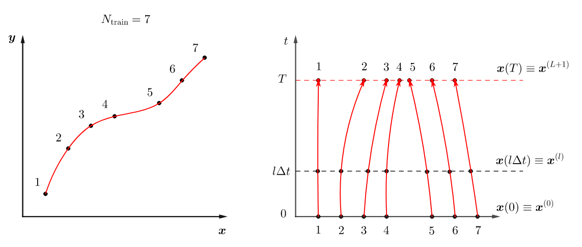
How do we use neural ODEs to solve a regression problem? Assume that you are given the labelled training data $\mathcal{S} = (x_j,y_j)_{1\leq j \leq N_{\text{train}}}$. Both, $x_j$ and $y_j$, are assumed to have the same dimension $d-1$. The key idea is to think of $x_j$ as points in $d-1$-dimensional space that represent the initial state of the system and $y_j$ as points that represent the final state. Then the regression problem becomes finding the dynamics, that is the RHS, of (2) that will map the initial to the final points with minimal error. This means finding the parameters $\theta$ such that

is minimal. Here, $x_j(T;\theta)$ is the solution at time $t=T$ to (2) with initial condition $x(0)=x_j$ and the RHS is represented by a feed-forward neural network $V(x,t;\theta)$.

ResNets vs. Neural ODEs

• If we interpret the number of time steps in a neural ODE as the number of hidden layers $L$ in a ResNet, then the computational cost for both methods is $\mathcal{O}(L)$. This is the cost associated with performing one forward propagation and one backward propagation. However, the memory cost associated with storing the weights of each layer, is different. For a neural ODE all weights are associated with the feed-forward network representing $V(x, t; \theta)$. Thus, the number of weights are independent of the number of time steps used to solve the ODE. On the other hand, for a ResNet the number of weights increases linearly with the number of layers, therefore the cost of storing them scales as $\mathcal{O}(L)$.

• With a neural ODE we can take the limit $\Delta t \to 0$ and study the converge since the size of the network remains unchanged. This is not feasible for ResNets where $\Delta t \to 0$ corresponds to network depth $L \to \infty$.

• ResNet uses a forward Euler type method, but with neural ODEs any type of numerical ODE solver is feasible. Consider, for example, higher-order explicit time-integrator schemes like the Runge-Kutta methods that converge to the true solution at a faster rate.

Example: Test Equation

Fit a neural network on the dynamics of the following ODE system with initial value.

The original equations are unknown to the neural network. The data set only consists of samples behaving in time like the ODE system describes. Feel free to train the model with more epochs for better results on your own machine.

using OrdinaryDiffEq
using DiffEqFlux, PlotlyJS

u0 = Float32[2.; 0.]
n_samples = 16
tspan = (0.0f0, 1.5f0)

function trueODEfunc(du, u, p, t)
    true_A = [-0.1 2.0; -2.0 -0.1]
    du .= ((u.^3)'true_A)'
end
t = range(tspan[1], tspan[2], length=n_samples)
prob = DiffEqFlux.ODEProblem(trueODEfunc, u0, tspan)
ode_data = Array(solve(prob, Tsit5(), saveat=t))

model = Chain(
    x -> x.^3,
    Dense(2, 50, tanh),
    Dense(50, 2),
)

n_ode = NeuralODE(model, tspan, Tsit5(), saveat=t, reltol=1e-7, abstol=1e-9)
ps = Flux.params(n_ode)

loss_n_ode() = sum(abs2, ode_data .- n_ode(u0))

data = Iterators.repeated((), 25)  # epochs

Flux.train!(loss_n_ode, ps, data, ADAM(0.1))
pred = n_ode(u0)

traces = [
    scatter(x=t, y=ode_data[1, :], name="u_1", mode="lines+markers"),
    scatter(x=t, y=ode_data[2, :], name="u_2", mode="lines+markers"),
    scatter(x=t, y=pred[1, :], name="u_1 pred", mode="lines+markers"),
    scatter(x=t, y=pred[2, :], name="u_2 pred", mode="lines+markers"),
]

plt = plot(traces)

We are not learning a solution to the original ODE. Instead, we are learning the tiny ODE system from which the ODE solution is generated. The neural network inside the neural ODE layer learns the function $u' = Au^3$. Thus, it learned a compact representation of how the time series behaves, and it can easily extrapolate to what would happen with different initial conditions. It is also a very flexible method for learning such representations if your data is unevenly spaced. Just pass in the desired time steps and the ODE solver takes care of it.

Exercise

Model the dynamics of the Lotka-Volterra system using a neural ODE. Refer to the Julia code above for help. See also notebooks/neural_ode.jl.

References

• Ray, Pinti and Oberai, Deep Learning and Computational Physics (Lecture Notes), 2023, https://arxiv.org/pdf/2301.00942.pdf.

• He, Zhang, Ren and Sun, Deep Residual Learning for Image Recognition, 2015, https://arxiv.org/pdf/1512.03385.pdf.

• Chen, Rubanova, Bettencourt and Duvenaud, Neural Ordinary Differential Equations, 2019, https://arxiv.org/pdf/1806.07366.pdf.

• Rackauckas, Innes, Ma, Bettencourt, White and Dixit, DiffEqFlux.jl – A Julia Library for Neural Differential Equations, 2019, https://julialang.org/blog/2019/01/fluxdiffeq/.