Numerical Methods

Introduction

While analytical solutions are available for solving simple DEs, they are rare for complex real-world problems. Numerical methods are techniques that enable us to tackle a vast spectrum of DEs, spanning from the elementary to the highly intricate. We will explore the principles of discretization, numerical integration, and iterative algorithms that form the backbone of these methods. With a focus on practicality, we will guide you through the process of selecting the most appropriate numerical method for various problem types, implementing them effectively, and interpreting the results accurately.

Throughout this chapter, we will navigate through ordinary differential equations (ODEs) and partial differential equations (PDEs), each presenting its unique set of challenges and opportunities. From the classic Euler's method to advanced finite element analysis, you will gain insights into a diverse array of numerical tools and their applications, ultimately equipping you with the skills to tackle a wide range of real-world problems.

The Problem

Given is an IVP of a first-order DE of the form

where $f\colon [x_0, \infty) \times \mathbb R^d$ is a function and the initial condition $y_0\in \mathbb R^d$ is a given vector. Assuming that the true solution $y(x)$ to (1) cannot be found (easily) we would like to construct a numerical approximation $\hat y(x)$ that is accurate enough, i.e., $y(x) \approx \hat y(x)$ in some sense.

Euler Method

One way of approximating the solution to (1) is to use tangent lines. From the definition of direction fields we know that any solution to an IVP must follow the flow of these tangent lines. Hence, a solution curve must have a shape similar to these lines. We use the linearization of the unknown solution $y(x)$ of (1) at $x=x_0$

The graph of this linearization is a straight line tangent to the graph of $y=y(x)$ at the point $(x_0, y_0)$. We now let $h>0$ be an increment of the $x$-axis. Then by replacing $x$ by $x_1 = x_0 + h$ in (2), we get

where $y_1 = L(x_1)$. The point $(x_1, y_1)$ on the tangent line is an approximation to the true solution $(x_1, y(x_1))$ on the solution curve. The accuracy of the approximation $L(x_1) \approx y(x_1)$ or $y_1\approx y(x_1)$ depends heavily on the size of the increment $h$ and the smoothness of $y$. Usually, the step size $h$ is chosen to be reasonably small.

By identifying the new starting points as $(x_1, y_1)$ with $(x_0, y_0)$ in the above discussion, we obtain an approximation $y_2 \approx y(x_2)$ corresponding to two steps of length $h$ from $x_0$, that is, $x_2 = x_1 + h = x_0 + 2h$, and

Continuing in this manner, we see that $y_1, y_2, y_3, \ldots$, can be defined recursively by the general formula for Euler's Method

where $x_n = x_0 + nh$, $n=0, 1, 2, \ldots$.

Example: Approximate Nonlinear ODE

Consider the IVP $y'=0.1\sqrt{y} + 0.4x^2$, $y(-2) = 1$. We are going to use Euler's method to obtain an approximation using first $h=1.0$ and then $h=0.5$.

using Plots
gr()

function euler(f, x0, xn, y0, n)
    h = (xn - x0)/n
  
    xs = zeros(n+1)
    ys = zeros(n+1)
  
    xs[1] = x0
    ys[1] = y0
  
    for i in 1:n
      xs[i + 1] = xs[i] + h
      ys[i + 1] = ys[i] + h * f(xs[i], ys[i])
    end
  
    return xs, ys
end

f(x, y) = 0.1*√y + 0.4*x^2

x_0 = -2
x_n = 2
y_0 = 0.5

h_1 = 1.0
h_2 = 0.5

n_1 = floor(Int, (x_n-x_0) / h_1)
n_2 = floor(Int, (x_n-x_0) / h_2)

plt = plot()
xs, ys = euler(f, x_0, x_n, y_0, n_1)
plot!(xs, ys, label="h=1.0", marker=(:circle))

xs, ys = euler(f, x_0, x_n, y_0, n_2)
plot!(xs, ys, label="h=0.5", marker=(:rect))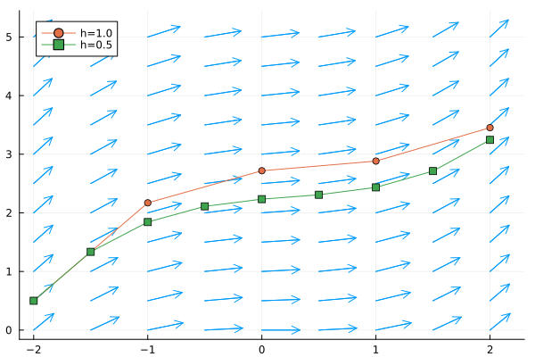

Euler’s method is just one of many different ways in which a solution of a DE can be approximated. Although attractive for its simplicity, Euler’s method is seldom used in serious calculations. It was introduced here simply to give you a first taste of numerical methods. We will go into greater detail in discussing numerical methods that give significantly greater accuracy.

Runge-Kutta Methods

Probably one of the more popular as well as most accurate numerical procedures used in obtaining approximate solutions to a first-order IVP $y'=f(x, y)$, $y(x_0) = y_0$ is the fourth-order Runge-Kutta (RK) method. As the name suggests, there are RK methods of different orders. RK methods are a class of methods which uses the information on the slope at more than one point to extrapolate the solution to future time step.

Motivation

Assume a function $y(x)$ is $k+1$ times continuously differentiable on an open interval containing $a$ and $x$. Then the Taylor polynomial can be used to write

where $c$ is some number between $a$ and $x$. After replacing $a$ and $x$ by $x_n$ and $x_{n+1} = x_n +h$, respectively, the formula turns into

where $c\in (x_n, x_{n+1})$. When $y(x)$ is a solution to $y'=f(x,y)$ in the case $k=1$ and the remainder $h^2/2y''(c)$ is close to 0, we see that the Taylor polynomial $y(x_{n+1}) = y(x_n) + hy'(x_n)$ of degree one agrees with the approximation formula of Eulers' method (3). Parameters of $m$-order RK methods are chosen such that they agree with a Taylor polynomial of degree $m$.

Second-Order Runge-Kutta Method

To further illustrate the motivation behind RK methods we derive a second-order RK procedure from scratch. Euler's method approximates $y(x_{n+1})$ with the derivative $f(x_n, y_n)$ which we call $k_1$ from now on. To get a better approximation we would like to incorporate the derivative at the halfway point between $x_n$ and $x_{n+1} = x_n + h$ labeled $k_2$. The problem is we do not know the exact value of $y(x_n + h / 2)$ so we also cannot find the exact value of $k_2$ at $x_n + h/2$. Instead, we approximate $y(x_n + h/2)$ using a first-order RK method and use it to approximate the slope at the midpoint $k_2$. The algorithm is outlined below.

1. Estimate derivative $k_1 = f(x_n, y_n)$

2. Approximate function at midpoint $y(x_n + h/2) \approx y_n + k_1 h / 2 = y^*$

3. Estimate slope at midpoint $k_2 = f(x_n + h/2, y^*)$

4. Final approximation $y(x_{n+1}) \approx y_{n+1} = y_n + k_2 h$

We can further generalize this concept by replacing the midpoint with fractional values $\alpha,\beta\in [0,1]$. The approximations of the derivative and the update equation are then defined as

Note that instead of only using one approximation of the derivative we now update the value with an average of both approximations. The previous method is described by $\alpha=\beta = 1/2$, but other choices are possible as well. The goal is to find values $w_1, w_2, \alpha, \beta$ such that the resulting error is low. Computing the two-dimensional Taylor series of $f(x,y)$ to expand the $k_2$ term yields

After plugging this back into (5) we get

Now we compare this expression to the Taylor polynomial of the exact solution given in (4). Note that according to the chain rule it holds that

They agree up to the error terms if we define the constants $w_1, w_2, \alpha$ and $\beta$ such that

This system has more than one solution since there are four unknowns and only three equations. Clearly the choice we made in the algorithm above with $w_1=0$ and $w_2=1$ and $\alpha = \beta = 1/2$ is one of these solutions. The local error of this method is $\mathcal{O}(h^3)$, hence the term second-order RK.

Generalization

The slope function $f$ is replaced by a weighted average of slopes over the interval $x_n \leq x \leq x_{n+1}$. That is,

Here, the weights $w_j, j=1, 2, \ldots, m$, are constants that generally satisfy $\sum_j w_j = 1$, and each $k_j,j=1, 2, \ldots, m$ is the function $f$ evaluated at a selected point $(x,y)$ for which $x_n \leq x \leq x_{n+1}$. The $k_j$ are defined recursively like

and the number $m$ is called the order of the method. By taking $m=1$, $w_1=1$, and $k_1 = f(x_n, y_n)$, we get the same formula as in (3). Hence, Euler's method is in fact just a first-order RK method. The characterics coefficients $c_j, a_{j\ell}$, and $w_j$ can be neatly arranged in the RK or Butcher tableau.

Example: Comparing Solvers

We compare the performance of various numerical methods on the simple harmonic oscillator problem given by

The classical RK4 method is given by the following tableau.

using OrdinaryDiffEq, PlotlyJS

# parameters
ω = 1

# initial conditions
x₀ = [0.0]
dx₀ = [π/2]
tspan = (0.0, 2π)
ts = 0:0.05:2π

# known analytical solution
ϕ = atan((dx₀[1] / ω) / x₀[1])
A = √(x₀[1]^2 + dx₀[1]^2)
truesolution(t) = @. A * cos(ω * t - ϕ)

# define the problem
function harmonicoscillator(ddu, du, u, ω, t)
    return @. ddu = -ω^2 * u
end
prob = SecondOrderODEProblem(harmonicoscillator, dx₀, x₀, tspan, ω)

# pass to solvers
midpoint = solve(prob, Midpoint())
rk4 = solve(prob, RK4())
tsit5 = solve(prob, Tsit5())

# plot results
traces = [
    PlotlyJS.scatter(x=ts, y=truesolution(ts), name="true", mode="lines"),
    PlotlyJS.scatter(x=midpoint.t, y=last.(midpoint.u), name="midpoint", mode="lines+markers"),
    PlotlyJS.scatter(x=rk4.t, y=last.(rk4.u), name="rk4", mode="lines+markers"),
    PlotlyJS.scatter(x=tsit5.t, y=last.(tsit5.u), name="tsit5", mode="lines+markers"),
]
plt = PlotlyJS.plot(traces)

As the numerical solvers grow in complexity from top to bottom the adaptive number of steps is reduced drastically. For a full list of available solvers for ODE problems we refer to https://docs.sciml.ai/DiffEqDocs/stable/solvers/ode_solve/ in the DifferentialEquations.jl package.

References

• Dennis G. Zill, A First Course in Differential Equations with Modeling Applications, 2018.