Differential Equations

Introduction

Differential equations promote the understanding and modeling of a multitude of phenomena in the natural world. These include the growth of populations, the behavior of subatomic particles, or thermal conduction, just to name a few examples. They provide a powerful mathematical framework for describing change and dynamics in diverse fields such as physics, engineering, biology, economics, and more. In this chapter we focus on two fundamental categories: ordinary differential equations (ODEs) and partial differential equations (PDEs).

Differential equations are mathematical expressions that describe how a function changes with respect to one or more independent variables. ODEs deal with functions of a single variable, encapsulating phenomena that evolve in one dimension, while PDEs are concerned with functions of multiple variables, allowing us to investigate systems that evolve, usually over time, in two or more dimensions. Together, ODEs and PDEs are indispensable tools for understanding and predicting the behavior of dynamic systems.

Definitions and Terminology

The derivative $\mathrm{d} y / \mathrm{d} x$ of a function $y(x)$ is itself another function $y'(x)$ found by an appropriate rule. Consider the exponential function $y(x) = \mathrm{e}^{0.1x^2}$ for example. It is differentiable on the interval $(-\infty, \infty)$ and by the chain rule its first derivative is given by $\mathrm{d} y(x) / \mathrm{d} x = 0.2x\mathrm{e}^{0.1x^2}$. If we plug in $y=y(x)$ on the right-hand side of this equation we get

$$\frac{\mathrm{d} y}{\mathrm{d} x} = 0.2 x y\,.$$

Now imagine that you are handed equation (1) and have no prior knowledge about $y$. Then the problem at hand can be formulated like this.

Equation (1) is called a differential equation. In general, any equation containing the derivatives of one or more unknown functions or dependent variables, with respect to one or more independent variables, is said to be a differential equation (DE).

Throughout this text ordinary derivatives will be written by using either the Leibniz notation $\mathrm{d} y / \mathrm{d} x$ or the prime notation $y'$. Using the latter DEs can be written a little more compactly. In physical sciences and engineering, Newton's dot notation $\dot y$ is also used to denote derivatives with respect to time. Partial derivatives are often denoted by a subscript notation $u_x$ indicating the independent variable $x$.

Classification

DEs can be classified according to type, order, and linearity.

Type: If a differential equation contains only ordinary derivatives of one or more unknown functions with respect to a single independent variable, it is said to be an ordinary differential equation (ODE). An equation involving partial derivatives of one or more unknown functions of two or more independent variables is called a partial differential equation (PDE).

Order: The order of either an ODE or a PDE is the order of the highest derivative in the equation. In symbols we can express an $n$-th-order ODE in one dependent variable by the general form

$$F(x,y,y',\ldots,y^{(n)}) = 0\,,$$

where $F$ is a real-valued function of $n+2$ variables. Note, that without loss of generality to higher-order systems, we can restrict ourselves to first-order DEs. That is because any higher-order ODE can be inflated into a larger system of first-order equations by introducing new variables. For example, the second-order equation $y'' = -y$ can be rewritten as a system of two first-order equations

Linearity: An $n$-th-order ODE (2) is said to be linear if $F$ is linear in $y,y',\ldots,y^{(n)}$. A nonlinear ordinary differential equation is simply one that is not linear. Nonlinear functions of the dependent variable or its derivatives, such as $\sin y$ or $\mathrm{e}^{y'}$, cannot appear in a linear equation.

Solutions of an ODE

Any function $\phi$, defined on an interval $I$ and possessing at least $n$ derivatives that are continuous on $I$, which when substituted into an $n$-th-order ODE reduces the equation to an identity, is said to be a solution of the equation on the interval. In other words, a solution of an $n$-th-order ODE (2) is a function $\phi$ that possesses at least $n$ derivatives and for which

We say that $\phi$ satisfies the differential equation on $I$. For our purposes we shall also assume that a solution $\phi$ is a real-valued function.

When solving a first-order differential equation $F(x, y, y')$ we usually obtain a solution containing a single constant or parameter $c$. A solution of $F(x, y, y')$ containing a constant $c$ is a set of solutions called a one-parameter family of solutions. When solving an $n$-th-order differential equation $F(x, y, y', \ldots, y^{(n)})$ we seek an $n$-parameter family of solutions. This means that a single differential equation can possess an infinite number of solutions corresponding to an unlimited number of choices for the parameter(s). A solution of a differential equation that is free of parameters is called a particular solution.

Systems of DEs

Often in theory, as well as in many applications, we deal with systems of DEs. A system of ODEs is two or more equations involving the derivatives of two or more unknown functions of a single independent variable. For example, if $x$ and $y$ denote dependent variables and $t$ denotes the independent variable, then a system of two first-order differential equations is given by

A solution of such a system is a pair of differentiable functions $x = \phi_1(t), y = \phi_2(t)$, defined on a common interval $I$, that satisfy each equation of the system on this interval.

Initial-Value Problems

We are often interested in problems in which we seek a solution $y(x)$ of a DE so that $y(x)$ also satisfies certain prescribed side conditions, that is, conditions that are imposed on the unknown function $y(x)$ and its derivatives at a number $x_0$. On some interval $I$ containing $x_0$ the problem of solving an $n$-th-order DE subject to $n$ side conditions specified at $x_0$

where $y_0,y_1, \ldots, y_{n-1}$ are arbitrary constants, is called an $n$-th-order initial-value problem (IVP). The values of $y(x)$ and its first $n-1$ derivatives at $x_0, y(x_0)=y_0, y'(x_0)=y_1, \ldots, y^{(n-1)}(x_0) = y_{n-1}$ are called initial conditions (ICs). Solving an $n$-th-order IVP frequently entails first finding an $n$-parameter family of solutions of the DE and then using the ICs at $x_0$ to determine the $n$ constants in this family. The resulting particular solution is defined on some interval $I$ containing the number $x_0$.

Geometric Interpretation

Consider the second-order IVP

We want to find a solution $y(x)$ of the DE $y'' - f(x,y,y')$ on an interval $I$ containing $x_0$ such that its graph not only passes through $(x_0,y_0)$ bu the slope of the curve at this point is the number $y_1$. A solution curve is shown in blue in the following Figure.

The words initial conditions derive from physical systems where the independent variable is time $t$ and where $y(t_0) - y_0$ and $y'(t_0)-y_1$ represent the position and velocity, respectively, of an object at some beginning, or initial, time $t_0$.

Example: Falling Bodies

To construct a mathematical model of the motion of a body moving in a force field, one often starts with the laws of motion formulated by the English mathematician Isaac Newton. Recall from elementary physics that Newton’s first law of motion states that a body either will remain at rest or will continue to move with a constant velocity unless acted on by an external force. In each case this is equivalent to saying that when the sum of the forces $F = \sum F_k$, the so-called net or resultant force, acting on the body is zero, then the acceleration $a$ of the body is zero. Newton's second law of motion indicates that when the net force acting on a body is not zero, then the net force is proportional to its acceleration $a$ or, more precisely, $F = ma$, where $m$ is the mass of the body.

Now suppose a baseball is tossed upward from the roof of a tall building. What is the position $s(t)$ of the baseball relative to the ground at time $t$? The acceleration of the baseball is the second derivative $\mathrm{d}^2 s / \mathrm{d} t^2$. If we assume that the upward direction is positive and that no force acts on the baseball other than the force of gravity, then Newton’s second law gives

In other words, the net force is simply the weight $F = F_1 = −W$ of the baseball near the surface of the Earth. Recall that the magnitude of the weight is $W = mg$, where $m$ is the mass of the body and $g$ is the acceleration due to gravity. The minus sign is used because the weight of the baseball is a force directed downward, which is opposite to the positive direction. If the height of the building is $s_0$ and the initial velocity of the baseball is $v_0$, then $s$ is determined from the second-order IVP

$$\frac{\mathrm{d}^2 s}{\mathrm{d} t^2} = -g\,,\quad s(0) = s_0\,,\quad s'(0) = v_0\,.$$

This can easily be solved by integrating the constant $−g$ twice with respect to $t$. The ICs determine the two constants of integration which yields

Using Julia we can formulate this problem and solve it numerically.

using OrdinaryDiffEq, PlotlyJS

# parameters
g = 9.81  # earth's gravity

# initial conditions
s₀ = [55.86]  # Leaning Tower of Pisa [m]
ds₀ = [20.0]  # average baseball throw [m/s]
tspan = (0.0, 7.0)  # time [s]

# define the problem
fallingbody!(dds, ds, s, p, t) = @. dds = -g

# pass to solvers
prob = SecondOrderODEProblem(fallingbody!, ds₀, s₀, tspan)
sol = solve(prob, DPRKN6(); saveat=0.5)

# define analytical solution
trueposition(t) = @. -1/2*g*t^2 + ds₀*t + s₀

# plot results
layout = Layout(;
    xaxis_title="Time [s]",
    yaxis_title="Position [m]",
)
trace1 = scatter(x=sol.t, y=max.(0, trueposition(sol.t)), name="true", mode="lines")
trace2 = scatter(x=sol.t, y=max.(0, last.(sol.u)), name="numerical")
plt = plot([trace1, trace2], layout)

In the model given in (3) the resistive force of air was ignored. Under some circumstances a falling body of mass $m$, such as a feather with low density and irregular shape, encounters air resistance proportional to its instantaneous velocity $v$. If we take the positive direction to be oriented upward, then the net force acting on the mass is given by $F = F_1 + F_2 = -mg + kv$, where the weight $F_1 = -mg$ of the body is force acting in the negative direction and air resistance $F_2 = kv$ is a force, called viscous damping, acting in the opposite or upward direction. Now, since $v$ is related to acceleration $a$ by $a = \mathrm{d} v / \mathrm{d} t$, Newton’s second law becomes $F = ma = m \mathrm{d} v / \mathrm{d} t$. By equating the net force to this form of Newton’s second law, we obtain a first-order DE for the velocity $v(t)$ of the body at time $t$

Here $k$ is a positive constant of proportionality. If $s(t)$ is the distance the body falls in time $t$ from its initial point of release, then $v=\mathrm{d} s / \mathrm{d} t$ and $a = \mathrm{d} v / \mathrm{d} t = \mathrm{d}^2 s / \mathrm{d} t^2$. In terms of $s$ this yields a second-order DE

We can adapt the Julia code snippet above to also account for the viscous damping factor.

using OrdinaryDiffEq, PlotlyJS

# parameters of Apollo 15 experiment
g = 9.81  # earth's gravity
k = 1.0
m_feather = 0.03  # [kg]
m_hammer = 1.32  # [kg]

# initial conditions
s₀ = [55.86]  # Leaning Tower of Pisa [m]
ds₀ = [0.0]  # drop [m/s]
tspan = (0, 15)  # [s]

# define the problems
function fallingbodyair!(dds, ds, s, p, t)
    k, m = p

    return @. dds = -m*g + k*ds
end

# pass to solvers
prob = SecondOrderODEProblem(fallingbodyair!, ds₀, s₀, tspan, [k, m_feather])
sol_feather = solve(prob, DPRKN6(); saveat=0.1)
prob = SecondOrderODEProblem(fallingbodyair!, ds₀, s₀, tspan, [k, m_hammer])
sol_hammer = solve(prob, DPRKN6(); saveat=0.1)

# plot results
layout = Layout(;
    xaxis_title="Time [s]",
    yaxis_title="Position [m]",
)

trace1 = scatter(x=sol_feather.t, y=max.(0, last.(sol_feather.u)), name="feather")
trace2 = scatter(x=sol_hammer.t, y=max.(0, last.(sol_hammer.u)), name="hammer")

plt = plot([trace1, trace2], layout)

Direction Fields

Let us assume that for some first-order DE $\mathrm{d} y / \mathrm{d} x = f(x, y)$ we can neither find a solution nor invent a method for solving it analytically. This is not as bad a predicament as one might think, since the DE itself can be used to investigate how its solutions “behave”. Even if an analytical or numerical solution has been found this qualitative analysis can be used to confirm the results. Direction fields tell us, in an approximate sense, what a solution curve must look like without actually solving the equation.

If we systematically evaluate $f$ over a rectangular grid of points in the $xy$-plane and draw a line element at each point $(x, y)$ of the grid with slope $f(x, y)$ like the vector

then the collection of all these line elements is called a direction field or a slope field of the DE. Visually, the direction field suggests the appearance or shape of a family of solution curves of the DE, and consequently, it may be possible to see at a glance certain qualitative aspects of the solutions, e.g., regions in the plane, in which a solution exhibits an unusual behavior. A single solution curve that passes through a direction field must follow the flow pattern of the field. It is tangent to a lineal element when it intersects a point in the grid. The Figure below shows a direction field of the DE $\mathrm{d} y / \mathrm{d} x = 0.2xy$ over a region of the $xy$-plane.

using Plots
gr()

xs, ys, us, vs = [], [], [], []
f(x, y) = 0.2*x*y

space = -5:1.0:5

for x in space, y in space
    push!(xs, x), push!(ys, y)

    v = f(x, y)
    norm = (1 + v^2)^(1/2)

    push!(us, 1 / norm), push!(vs, v / norm)
end

quiver(xs, ys, quiver=(us, vs))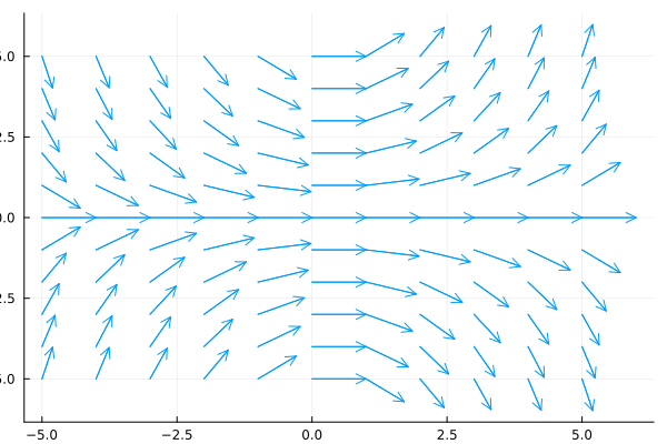

Systems of DEs

We have seen that a single DE can serve as a mathematical model for a single population in an environment. But if there are, say, two interacting and perhaps competing species living in the same environment (for example, rabbits and foxes), then a model for their populations $x(t)$ and $y(t)$ might be a system of two first-order DE such as

$$\begin{aligned} \frac{\mathrm{d} x}{\mathrm{d} t} &= g_1(t, x, y)\,, \\ \frac{\mathrm{d} y}{\mathrm{d} t} &= g_2(t, x, y)\,. \end{aligned}$$

When $g_1$ and $g_2$ are linear in the variables $x$ and $y$ then (4) is said to be a linear system.

General Definition

Let $\Omega \subset \mathbb R \times (\mathbb R^m)^{n+1}$, $n\in\mathbb N$, and $f\colon \Omega \to \mathbb R^m$ continuous. Then

is called an explicit system of ordinary differential equations of order $n$. The implicit analogue is given by

Example: Lotka-Volterra Model

Suppose two different species of animals interact within the same environment or ecosystem. Suppose further that the first species eats only vegetation and the second eats only the first species. In other words, one species is the predator, and the other is prey. For example, wolves hunt grass-eating caribou, sharks devour little fish, and the snowy owl pursues an arctic rodent called the lemming. For the sake of discussion, let us imagine that the predators are foxes and the prey are rabbits. Let $x(t)$ and $y(t)$ denote the fox and rabbit populations, respectively, at time $t$. If there were no rabbits, then one might expect that the foxes, lacking an adequate food supply, would decline in number according to

$$\frac{\mathrm{d} x}{\mathrm{d} t} = -ax\,,\quad x > 0\,.$$

When rabbits are present in the environment, however, it seems reasonable that the number of encounters or interactions between these two species per unit time is jointly proportional to their populations $x$ and $y$., i.e., proportional to the product $xy$. Thus, when rabbits are present, there is a supply of food, so foxes are added to the system at a rate $bxy$, $b>0$. Adding this last rate to (5) gives a model of the fox population

On the other hand, if there were no foxes, then the rabbits would, with an added assumption of unlimited food supply, grow at a rate that is proportional to the number of rabbits present at time $t$

But when foxes are present, a model for the rabbit population is this equation decreased by $cxy$, $c>0$, that is, decreased by the rate at which the rabbits are eaten during their encounters with the foxes

This constitutes the system of nonlinear DEs

where $a,b,c$, and $d$ are positive constants. This famous system of equations is known as the Lotka-Volterra predator-prey model.

using OrdinaryDiffEq, PlotlyJS

function lotka_volterra(du, u, params, t)
    🐰, 🐺 = u
    α, β, δ, γ = params
    du[1] = d🐰 = α*🐰 - β*🐰*🐺
    du[2] = d🐺 = -δ*🐺 + γ*🐰*🐺
end

u0 = [1.0, 1.0]
tspan = (0.0, 15.0)
params = [1.5, 1.0, 3.0, 1.0]

prob = ODEProblem(lotka_volterra, u0, tspan, params)
sol = solve(prob, Tsit5(); saveat=0.2)

# plot results
layout = Layout(;
    xaxis_title="Time [d]",
    yaxis_title="Number",
)

rabbits = scatter(x=sol.t, y=first.(sol.u), name="rabbits")
wolves = scatter(x=sol.t, y=last.(sol.u), name="wolves")

plt = plot([rabbits, wolves], layout)

Exercise

Model the spread of a contagious disease using the compartmental SIR model from epidemiology. See also notebooks/contagious_disease.jl.

Partial Differential Equations

An ODE describes the relation between an unknown function depending on a single variable and its derivatives. A partial differential equation (PDE) describes a relation between an unknown function and its partial derivatives. PDEs appear frequently in all areas of physics and engineering. Moreover, in recent years we have seen a dramatic increase in the use of PDEs in areas such as biology, chemistry, computer sciences (particularly in relation to image processing and graphics) and in economics (finance). In fact, in each area where there is an interaction between a number of independent variables, we attempt to define functions in these variables and to model a variety of processes by constructing equations for these functions. When the value of the unknown function(s) at a certain point depends only on what happens in the vicinity of this point, we shall, in general, obtain a PDE. The general form of a PDE for a function $u(x_1, x_2, \ldots, x_n)$ is given by

$$F(x_1, x_2, \ldots, x_n, u, u_{x_1}, u_{x_2}, \ldots, u_{x_{11}}, \ldots) = 0\,,$$

where $x_1, x_2, \ldots, x_n$ are the independent variables, $u$ is the unknown function, and $u_{x_j}$ denotes the partial derivative $\partial u / \partial x_j$. Also partial derivatives of higher order like $\partial u / \partial x_{jk}$ are possible. The equation is, in general, supplemented by additional conditions such as initial conditions, as we have already seen in the theory of ODEs, or boundary conditions.

Classification

Similar to ODEs we can classify PDEs into different categories.

Order: The order is defined to be the order of the highest derivative in the equation. If the highest derivative is of order $k$, then the PDE is said to be of order $k$. Thus, for example, the equation $u_{tt} - u_{xx} = f(x,t)$ is called a second-order equation, while $u_t + u_{xxx} = 0$ is called a third-order equation.

Linearity: A PDE is called linear if in (6), $F$ is a linear function of the unknown function $u$ and all of its derivatives. For example, $x^7u_x + \mathrm{e}^{xy}u_y + \sin(x^2 + y^2)u= x^3$ is a linear equation while $u_x^2 + u_y^2=1$ is a nonlinear equation.

Scalar versus system: A single PDE with just one unknown function is called a scalar equation. In contrast, a set of $m$ equations with $\ell$ unknown functions is called a system of $m$ equations.

Example: Poisson's Equation

Poisson's equation is a second-order PDE frequently used in theoretical physics. Given the Laplace operator in $n$-dimensional space

it is defined by

where the initial condition $f$ is given and $\phi$ is the unknown solution.

References

• Dennis G. Zill, A First Course in Differential Equations with Modeling Applications, 2018.

• Simon Frost, SIR model in Julia using DifferentialEquations, 2018, http://epirecip.es/epicookbook/chapters/sir/julia.

• Pinchover and Rubinstein, An Introduction to Partial Differential Equations, 2005.